The 1D Wave
Contents
The 1D Wave#
Author: Matthew Hamilton, edits Andrew Gibbs
This example of FDTD in Python will consider the 1D Wave Equation with generic loss:
Assumptions#
This tutorial assumes that you are already familiar with the 1D Wave Equation and its derivation. It also assumes that you have a grasp of finite difference operators and the derivation of the finite difference scheme for the 1D Wave equation.
Who are you#
The assumed audience for this tutorial is someone who is familiar with the baic of python but has never programmed a finite difference scheme before. It is also relevant to those who are familiar with programming a finite difference scheme in MATLAB, but wish to create an implement in python.
Overview#
As a reminder, the finite difference scheme for the 1D wave we are trying to implement is:
with following defintions:
\(n\): the time step index
\(k\): time step for a given sample rate
\(\lambda\): the courant number
\(\sigma\): a loss parameter
\(A\), \(B\), and \(C\): coefficient matrices.
This of course is not the only way we can express the scheme, however a matrix approach will be taken for the remainder of this tutorial. This should hopefully provide a clear connection between the above equation of motion and the actuall programme. The scheme could also be expressed in terms of grid point \(l\), which is a perfectly legitmate method and it would be more relevant for a programme that does not take a matrix approach (e.g. C / C++):
Any Finite Difference scheme you need to programme can likely be split into the following sections:
-
Simluation Parameters
Defined Coefficients
Derived Coefficients
Grid Coefficients
-
Stencil Matrices
Coefficient Matrices
Time State Vector
Input Output Vectors
-
Initial Conditions
Main Time Loop
A full version of the script can be found in Appendex A. The following breakdown of the script will explore and elaborate on certain choices you might make that would be absent from a final verion.
Import Libraries#
from numpy import pi, log, sqrt, floor, zeros
from scipy import sparse
from IPython.display import Audio
We have decided here to import only specific functions from numpy. This will make some of the code more brief, but also provide more explicit parallels to what you may write in MATLAB / Octave. See numpy’s own style guide when using numpy in a larger code base.
scipy provides the functionality we need for sparse matrices. The style guide for scipy is to simply include the module that is required unlike numpy’s import numpy as np style.
The final import statement from IPython.display import Audio imports the Audio class for IPython, which whill provide a handy interface for listening to the output.
Parameters#
Next we will define the parameters which will provide our point of entry for interacting with the model.
Simulation Parameters#
The first set of parameters relate to the actual simulation. This section will contain parameters such as sample rate, duration, input and output points.
SR = 44100.0  # sample rate (Hz)
Tf = 1.0      # duration of simulation (s)
xi = 0.8      # coordinate of excitation (normalised, 0 - 1)
xo = 0.1      # coordinate of output (normalised, 0 - 1)
Coefficients#
The next set of parameters are the coefficients, which will be split into three cataegories
Defined
Derived
Grid
Defined#
Defined coefficients are those which you will give an actual explicit value. In this case we have:
f0: the fundamental frequency \(f_0\)r: the radius of the string in metersL: the length of the string in metersrho: the density \(\rho\) in \(\text{kg m}^{-3}\)T60: the \(T_{60}\) decay time
f0 = 110.0   # fundamental frequency (Hz)
r = 1.27e-4  # string radius (m)
L = 1.0      # length (m)
rho = 7850   # density (kg/m^3) of steel
T60 = 2.0    # T60 (s)
Derived#
The next set of coefficients are those which are derived from the previous set.
A definition of tension \(T\) based on the \(f_0\), density, length, and radius is included here for easier interaction with the programme.
T = ((2.0 * f0 * L * r) ** 2.0) * rho * pi  # Tension in Newtons
A = pi * (r ** 2.0)          # string cross-sectional area
c = sqrt(T / (rho * A))      # wave speed
sig = 6.0 * log(10.0) / T60  # loss parameter
To demarcate easily between float and int types it is recommendate to include the .0 on numbers where the value is intended to be a float.
Grid#
Grid coefficients are those that relate to the FDTD and not the physical model and include variables such as
k: the time step for a given sampling ratehmin: the minimume grid spacing \(h_{\text{min}}\) derived from von Neumann anaylsisN: number of grid points given a length \(L\) and \(h_{\text{min}}\)h: an adjusted grid spacing which depends onNand which will be used as the grid spacing for the remainderlamb: the courant number \(\lambda\)Nf: The number of time steps in the simulation which is derived from sampling rate and simulation duration \(T_f\)
k = 1.0 / SR  # time step
hmin = c * k  # stability condition

N = int(floor(L / hmin))  # number of segments (N+1 is number of grid points)
h = L / N                 # adjusted grid spacing

lamb = c * k / h          # Courant number
Nf = int(floor(SR * Tf))  # number of time steps
It is important to note that the simulation will not be stable unless \(h > h_{\text{min}}\)
Both N and Nf are integers, however the output of numpy’s floor function will be float given that L and hmin are float type variables. Wrapping the function in int() converts the type to integer, which is required when indexing an array.
The variable name lamb has been used as lambda is a reserved word in python.
Matrices#
Stencil Matrices#
For quality of life we can define some stencil matrices so that our calculations are similar to the update equation.
I = sparse.eye(N)
Dxx = sparse.diags([1, -2, 1], [-1, 0, 1], shape=(N, N))
It is worth noting here that if some boundary conditions were required, then the initialisation of Dxx would be a little different. The return format of sparse.diags is not fixed. If you need to make further alterations to the stencil, then you may need to specify a sparse matrix format.
Coefficient Matrices#
Reminding ourselves of the scheme:
with the coefficient matrices defined as:
We can tweak these definitions a little to be
Given all the ground work that has been done, we can now pretty much just write that.
A = 1.0 / (1.0 + (k * sig))  # inverted
B = A * ((lamb ** 2.0) * Dxx + (2.0 * I))
C = A * ((-1.0 + (k * sig)) * I)
A has been pre-inverted here to avoid some uglier formatting.
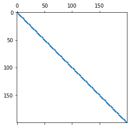
Stencil Shape#
It is good practice at this point to have a look at the shape the matrices. This will confirm if you need to make any adjustments or “zero out” any rows or columns in your matrices.
B Matrix#
import matplotlib.pyplot as plt

plt.spy(B, markersize=0.5)
plt.show()
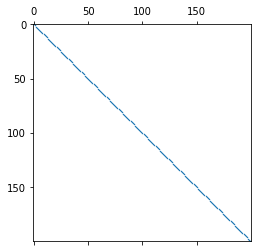
C Matrix#
plt.spy(C, markersize=0.5)
plt.show()
Time State Vectors#
Allocate the correct amount of memory using numpy’s zeros() function.
There are only 3 time steps in the scheme. This means we only need 3 vectors which we can swap each time step. The states in our scheme \(u^{n}\), \(u^{n-1}\), and \(u^{n-2}\) can be will be represented by u0, u1, and u2 respectively.
u0 = zeros(N)
u1 = zeros(N)
u2 = zeros(N)
Input / Output#
Here we can define our inputs and outputs. We want to get audio output of our simulation so we will need a vector of size Nf to hold our sample ouput for each time step.
We also need to define the grid point the initial condition will be placed, li, and the grid point that will be used as the audio “read-out” point, lo.
out = zeros(Nf)

li = int(floor(xi * N))  # grid index of excitation
lo = int(floor(xo * N))  # grid index of output
Since li and lo are indices, we use int here to convert the output of floor.
Simulation#
Initial Conditions#
The intial condition will be a simple delta.
u1[li] = 1.0
Main Time Loop#
for n in range(Nf):
    u0 = B * u1 + C * u2
    u2, u1, u0 = u1, u0, u2  # state swap
    out[n] = u0[lo]
The update u0 = B * u1 + C * u2 is pretty close to the original scheme equation.
The second step of swapping the states is a little less intuitive. Here we pack the states into a list on the right hand side:
= u1, u0, u2
We can then unpack the same list into the same variables on the left hand side
u2, u1, u0 =
u0 = u2u2 = u1u1 = u0
However if we were to write it this way
u0 = u2 # fine
u2 = u1 # fine
u1 = u0 # uh-oh, this means u1 == u2 !!
This is because assigning one numpy array variable to another does not copy it as you might expect in MATLAB.
After this we read u0 at index lo and store that as a sample at index n in our audio vector out.
After running the simulation we should be able to listen to out array using the Audio class
Audio(data=out, rate=SR)