Boundary Element Method - Computational Tutorial
Contents
Boundary Element Method - Computational Tutorial#
Author: Andrew Gibbs
You can run this code directly in your browser by clicking on the rocket logo ( ) at the top of the page, and clicking ‘Binder’. This will open a Jupyter Notebook in a Binder environment which is set up to contain everything you need to run the code. Don’t forget to save a local copy if you make any changes!
If you prefer, you can download the Jupyter Notebook file to run locally, by clicking the download logo ( ) at the top of the page and selecting ‘.ipynb’.
If you are new to using Jupyter Notebooks, this guide will help you get started.
Prerequisites#
To understand the basic principles explained in this tutorial, you should:
(Maths) Have an understanding of the exterior Helmholtz scattering problem
(Maths) Have a basic understanding of the midpoint rule, for approximating integrals
(Python) Be comfortable using
numpy
import numpy as np
import matplotlib.pyplot as plt
Step one: Obtain a representation for the solution in terms of boundary data#
Our starting point is the representation (4):
where \(\frac{\partial}{\partial n}\) denotes the outward normal derivative, \(\partial\Omega\) denotes the boundary of \(\Omega\), and \(\Phi\) denotes the fundamental solution
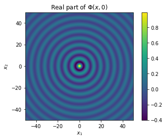
where \(H^{(1)}_0\) is the Hankel function of the first kind order zero. You probably recognise the function for \(n=3\), but if you haven’t seen \(H^{(1)}_0\) before, it looks like the ripples on the surface of a lake after you drop a pebble into the water:
from scipy.special import hankel1 as H1
t = np.linspace(-50, 50, 1000)
X, Y = np.meshgrid(t, t)
ripples = plt.imshow(np.real(H1(0, np.sqrt(X ** 2 + Y ** 2))), extent=[t.min(), t.max(), t.min(), t.max()])
plt.colorbar(ripples)
plt.title('Real part of $\\Phi(x,0)$')
plt.xlabel("$x_1$")
plt.ylabel("$x_2$")
Text(0, 0.5, '$x_2$')
For this simple example, we will consider scattering by a circle in two-dimensions, with sound-soft aka Dirichlet boundary conditions. This means that \(u=0\) on \(\partial\Omega\), so the BIE above simplifies to
The integral may be interpreted as lots of tiny speakers \(\Phi(x,y)\) on our surface \(\Gamma\), whilst \(\frac{\partial u}{\partial n}(y)\) can be interpreted as the volume of these speakers. We will choose our incoming wave to be an incident plane wave, \(u^i(x)=\mathrm{e}^{\mathrm{i} k x\cdot d}\), where \(d\in\mathbb{R}^2\) is a unit vector which represents the direction of propagation.
k = 5.0  # wavenumber
d = np.array([1.0, 0.0])  # incident direction
Phi = lambda x, y: 1j / 4 * H1(0, k * np.linalg.norm(np.array(x) - np.array(y)))
ui = lambda x: np.exp(1j * k * np.dot(x, d))
Step two: Reformulate as a problem on the boundary \(\Gamma\)#
Remember, our long-term aim is to approximate \(\frac{\partial u}{\partial n}\), then we can plug that approximation into the above equation, to obtain an approximation for \(u(x)\). To get an equation we can solve, we take the limit of the above equation as \(x\) tends to \(\Gamma\) and rearrange, to obtain a boundary integral equation (BIE), of the form (5):
A BEM is an approximation of an equation of this type, defined on the boundary \({\partial\Omega}\). Before approximating, we can parametrise the circle \({\partial\Omega}\) by \(\theta\in[0,2\pi)\to x\in{\partial\Omega}\) in the natural way, \(x(\theta)=[\cos(\theta),\sin(\theta)]\), to rewrite the above BIE in terms of a one-dimensional parameter
where \(\tilde\Phi(\theta,\vartheta):=\Phi(x(\theta),y(\vartheta))\) is purely to keep things a bit simpler. There are many BEMs, but for the purpose of this example, I will choose the simplest one I can think of.
circle_map = lambda theta: [np.cos(theta), np.sin(theta)]
ui_angular = lambda theta: ui(circle_map(theta))
Phi_tilde = lambda theta, vartheta: Phi(circle_map(theta), circle_map(vartheta))
Step three: Approximate the boundary data#
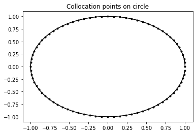
Choose \(N\) equispaced points on the circle \(\theta_n=nh\) where \(h:=2\pi/N\) for \(n=0,\ldots,N-1\). For our approximation, we specify that the above BIE must hold exactly at these points. This is known as a collocation BEM, and \(\theta_n\) are the collocation points:
where we choose the details of our approximation \(v^{(h)}(\theta)\approx\frac{\partial u}{\partial n}(y(\theta))\) next.
N = 80  # number of collocation points
theta = np.linspace(0, 2 * np.pi, N, endpoint=False)  # equispaced points on circle
h = 2 * np.pi / N  # meshwidth
plt.plot(np.cos(theta), np.sin(theta), 'k.-')
plt.title('Collocation points on circle')
Text(0.5, 1.0, 'Collocation points on circle')
We will use a piecewise constant approximation \(v^{(h)}(\theta)\), such that \(v^{(h)}(\theta)=v_m\) for \(\theta\in[\theta_m-h/2,\theta_m+h/2]\) and \(v^{(h)}(\theta)=0\) otherwise, for \(m=1,\ldots,N\). Note that the values \(v_m\) are currently unknown. A piecewise constant approximation is sometimes referred to as \(h\)-BEM. So the full name of this method is collocation \(h\)-BEM, and it can be expressed in the following form:
We can represent the above equation as a linear system for the unknowns \(v_m\):
where \(A_{mn}:=\int_{\theta_m-h/2}^{\theta_m+h/2}\tilde\Phi(\theta_m,\vartheta)~\mathrm{d}\vartheta\), and \(u_n := u^i(x(\theta_n))\). Even in this simple example, I hope it is clear that efficient methods for evaluating singular integrals play a key role in BEMs. The Nystrom variant of BEM is fast and simple (perfect for this example). The idea is to approximate (almost) each integral \(A_{mn}:=\int_{\theta_m-h/2}^{\theta_m+h/2}\tilde\Phi(\theta_n,\vartheta)~\mathrm{d}\vartheta\) by a one-point quadrature rule, which means we can use our collocation points as our quadrature points. This gives
where \(O(h^2)\) means the error is bounded above by \(Ch^2\), for some constant \(C\) and sufficiently small \(h\).
But we must be careful, a one-point quadrature rule for \(m=n\) gives \(h\Phi(\theta_n,\theta_m)=\infty\), since the Hankel function is unbounded at zero! So we need something a little more sophisticated for the diagonal elements.
From DLMF (10.4.3), (10.8.2), (10.2.2), we can consider the first term in the asymptotic expansion of the Hankel function, integrate the \(\log\) exactly, to write
where \(\gamma\approx0.577\) is Euler’s number and \(\epsilon\) is any number in \((0,1)\).
Now we can construct the matrix \(A\):
eulergamma = 0.57721566
singular_diagonal = lambda h: 1j * h * (2j * eulergamma + 2j * np.log(h * k / 4) + 1j * np.pi - 2j) / (4 * np.pi)
# construct matrix
A = np.zeros((N, N), dtype=complex)
for n in range(N):
for m in range(N):
if n == m:
A[m, n] = singular_diagonal(h)
else:
A[m, n] = h * Phi_tilde(theta[n], theta[m])
# construct right-hand side vector
u = np.zeros(N, dtype=complex)
for n in range(N):
u[n] = ui_angular(theta[n])
# solve linear system to get values of piecewise constant approximation:
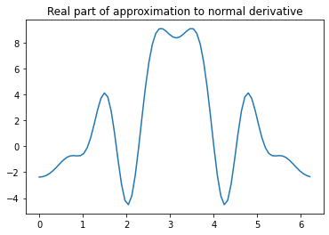
v = np.linalg.solve(A, u)
plt.plot(theta, np.real(v))
plt.title('Real part of approximation to normal derivative')
Text(0.5, 1.0, 'Real part of approximation to normal derivative')
Step four: Use approximate boundary data in representation formula#
Specifically: we will use the approximate boundary data from step three in the representation formula from step one.
Plugging \(v_h\) into the representation formula, and paramerising in the same way as before, gives
To be quick, we can use a one-point quadrature rule to evaluate this integral:
# create a method which approximates the solution at a point in the scattering domain
def sol_approx(x):
    val = ui(x)
    for n in range(N):
        val -= h * Phi(x, circle_map(theta[n])) * v[n]
    return val
num_pixels = 100
t = np.linspace(-3, 3, num_pixels)
X, Y = np.meshgrid(t, t)
u_h = np.zeros((num_pixels, num_pixels), dtype=complex)
for i in range(num_pixels):
for j in range(num_pixels):
if (X[i, j] ** 2 + Y[i, j] ** 2) > 1:
u_h[i, j] = sol_approx([X[i, j], Y[i, j]])
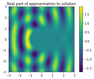
sol = plt.imshow(np.real(u_h), extent=[t.min(), t.max(), t.min(), t.max()])
plt.colorbar(sol)
plt.title('Real part of approximation to solution')
Text(0.5, 1.0, 'Real part of approximation to solution')