Finite Difference
Contents
Finite Difference#
Authors: Amelia Gully
Warning
This part of the site is currently under development.
The finite difference (FD) approach is one way of approximating a solution to a partial differential equation (PDE).
Approximating partial derivatives#
In a differential equation, we have one or more differential terms. Recall that a differential term describes a gradient, calculated over infinitestimally-small steps (i.e. \(\frac{\Delta x}{\Delta y}\) tends to \(\frac{\partial x}{\partial y}\)). A finite difference is a way of approximating the gradient by using steps of a known, finite size instead. We can then use this as an approximation to the true solution. To approximate a partial derivative we will replace the partial derivative terms in our equation with a finite-difference approximation to each of them.
For example, consider a first-order term like \(\frac{\partial u}{\partial t}\). This term represents the gradent of \(u\) with respect to \(t\). As such, we can approximate it by calculating the gradient between two points separated by a time step \(\Delta t\). Let us call those points \(u(t)\) and \(u(t-\Delta t)\). We calculate the gradient using \(\frac{u(t) - u(t - \Delta t)}{\Delta t}\) as shown below. By approximating the gradient this way, we do lose some detail, but we get a reasonable approximation if \(\Delta t\) is small enough.
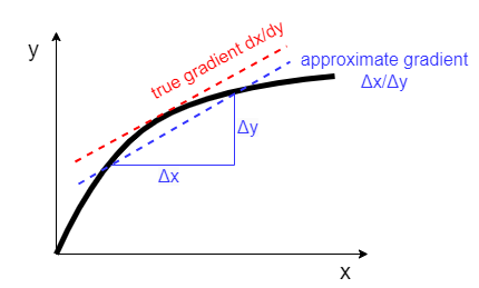
Fig. 6 Approximating the derivative with a simple gradient. Image credit: Amelia Gully 2024.#
Therefore, to obtain a finite difference approximation, of a partial derivative term like \(\frac{\partial u}{\partial t}\), we replace it with \(\frac{u(t) - u(t - \Delta t)}{\Delta t}\).
Types of difference#
You might notice here that we’re looking backwards in time; that is, if we are currently at time \(t\), we are approximating the gradient based on the difference between now and \(\Delta t\) seconds ago. This type of difference is therefore known as a backward difference.
We could also use a forward difference by looking forward in time \(\frac{u(t+\Delta t) - u(t)}{\Delta t}\), or we could take an interval centred on time \(t\) by using a central difference \(\frac{u(t+\frac{1}{2}\Delta t) - u(t-\frac{1}{2}\Delta t)}{\Delta t}\), depending on the requirements of our problem. If you’re not sure which to use, or it doesn’t matter for your application, the central difference is usually a reasonable place to start.
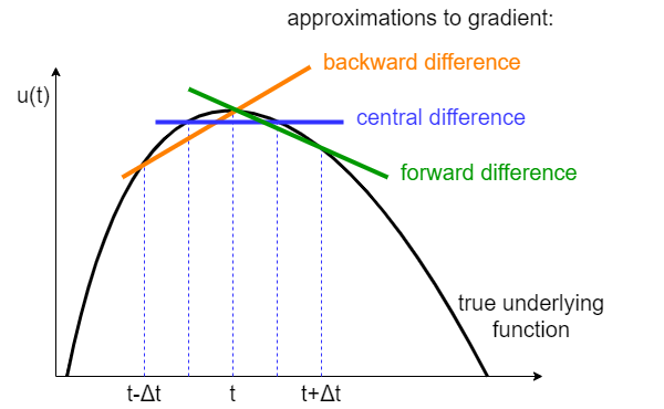
Fig. 7 Backward, central and forward differences. Image credit: Amelia Gully 2024.#
For second order differential terms, like \(\frac{\partial^2 u}{\partial t^2}\), we require a second-order finite difference term. Using a central difference we would replace \(\frac{\partial^2 u}{\Delta t^2}\) with \(\frac{u(t+\Delta t) - 2u(t) + u(t-\Delta t)}{\Delta t^2}\) (multiply out \((\frac{u(t+\frac{1}{2}\Delta t) - u(t-\frac{1}{2}\Delta t)}{\Delta t})^2\) to satisfy yourself that this is indeed a central difference term!)
Approximating the acoustic wave equation#
In acoustics, we are often dealing with the wave equation, so we will use this as an example here. The wave equation describes how acoustic pressure varies as a function of time (t) and space (x,y,z). For simplicity, let us consider only 1D wave propagation here, so spatial position is described by a single variable, x. We therefore denote acoustic pressure as \(u(x,t)\).
The 1D wave equation is constructed as follows (equivalent to the equation here, with only one spatial dimension):
\(\frac{\partial^2 u(x,t)}{\partial t^2} - \frac{1}{c^2} \frac{\partial^2 u(x,t)}{\partial x^2} = 0\)
We have two second-order partial derivatives, one in \(t\) and one in \(x\). We now know how to approximate these using finite differences. The finite difference approximation to the wave equation, using a central difference, therefore becomes:
\(\frac{u(x,t+\Delta t) - 2u(x,t) + u(x,t-\Delta t)}{\Delta t^2} - \frac{1}{c^2} \frac{u(x+\Delta x,t) - 2u(x,t) + u(x-\Delta x,t)}{\Delta x^2} = 0\)
Now we no longer require differentiation, so we can calculate an approximate solution given appropriate initial and boundary conditions.
Using the finite difference scheme#
To run a finite-difference simulation for the wave equation, we therefore define a set of spatial locations for x, and a set of time samples for t. We rearrange the above equation for \(u(x,t + \Delta t)\), so that we eventually obtain:
\(u(x,t+\Delta t) = (2-2\lambda^2)u(x,t) + \lambda^2(u(x+\Delta x,t)+u(x-\Delta x,t)) - u(x,t-\Delta t) \),
where \(\lambda = \frac{c\Delta t}{\Delta x}\) (see the information on the CFL condition for more information).
We can therefore calculate the pressure at point \(x\) for the next timepoint, \(u(x,t+\Delta t)\) based only on the pressures of point \(x\) and its neighbours \(x+1\) and \(x-1\) at the current and previous time points, \(t\) and \(t-\Delta t\). This is the basis of a finite-difference simulation.
Try it yourself#
To implement the finite difference scheme, try out our simple tutorials in one, two (coming soon!), and three (coming soon!) dimensions. These tutorials also explore how initial and boundary conditions are implemented and affect the simulation.