Why use Computational Acoustics?

Author: Jonathan Hargreaves, Amelia Gully

Warning

This part of the site is currently under development.

Computational acoustics (CA) describes the simulation of acoustic behaviour using computational techniques. In real situations, acoustic waves propagate and interact with their environments in a range of different ways. For simple sources, geometries and media, it may be possible to analytically determine (i.e. calculate) the acoustic behaviour of the system, but real-world sources and environments are often complicated and make analytical solutions impossible. Without computational acoustics, it would be neccesary to build such systems physically in order to determine how they behave acoustically. Computational acoustics allows us to model them virtually instead, which has a number of advantages that will be descibed below.

Note that computational acoustics techniques are approximations to the true acoustic behaviour. However, modern computational approaches are generally good enough to provide an accurate description of the acoustics of the equivalent physical system, given accurate information about the system’s properties.

Product Design Cycles

Traditional Physical Product Design Cycles

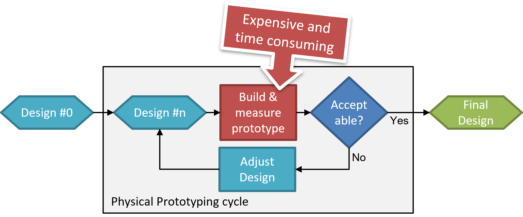
Fig. 1 Traditional Physical Product Design Cycles. Image credit: Jonathan Hargreaves

Simulation-Enhanced Product Design Cycles

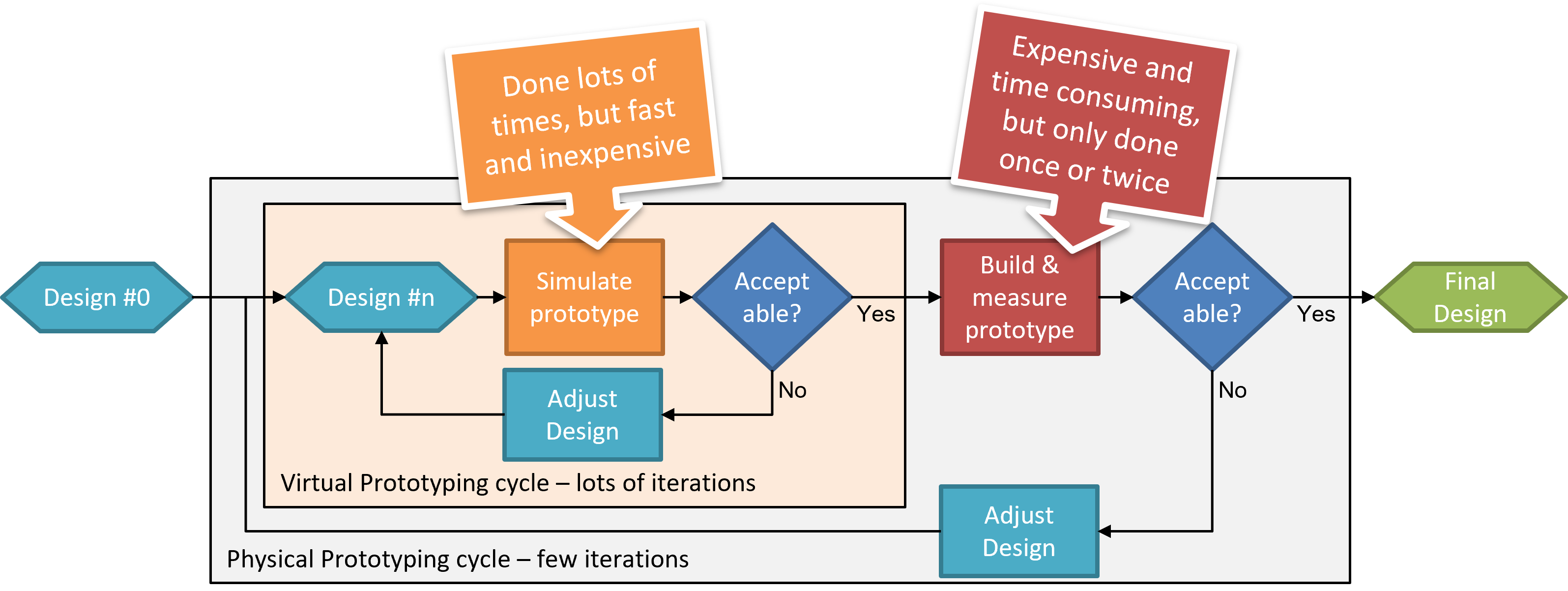
Fig. 2 Simulation-Enhanced Product Design Cycles. Image credit: Jonathan Hargreaves

Additional insight that would be challenging to measure

This example considers a Chladni plate.

Measurement

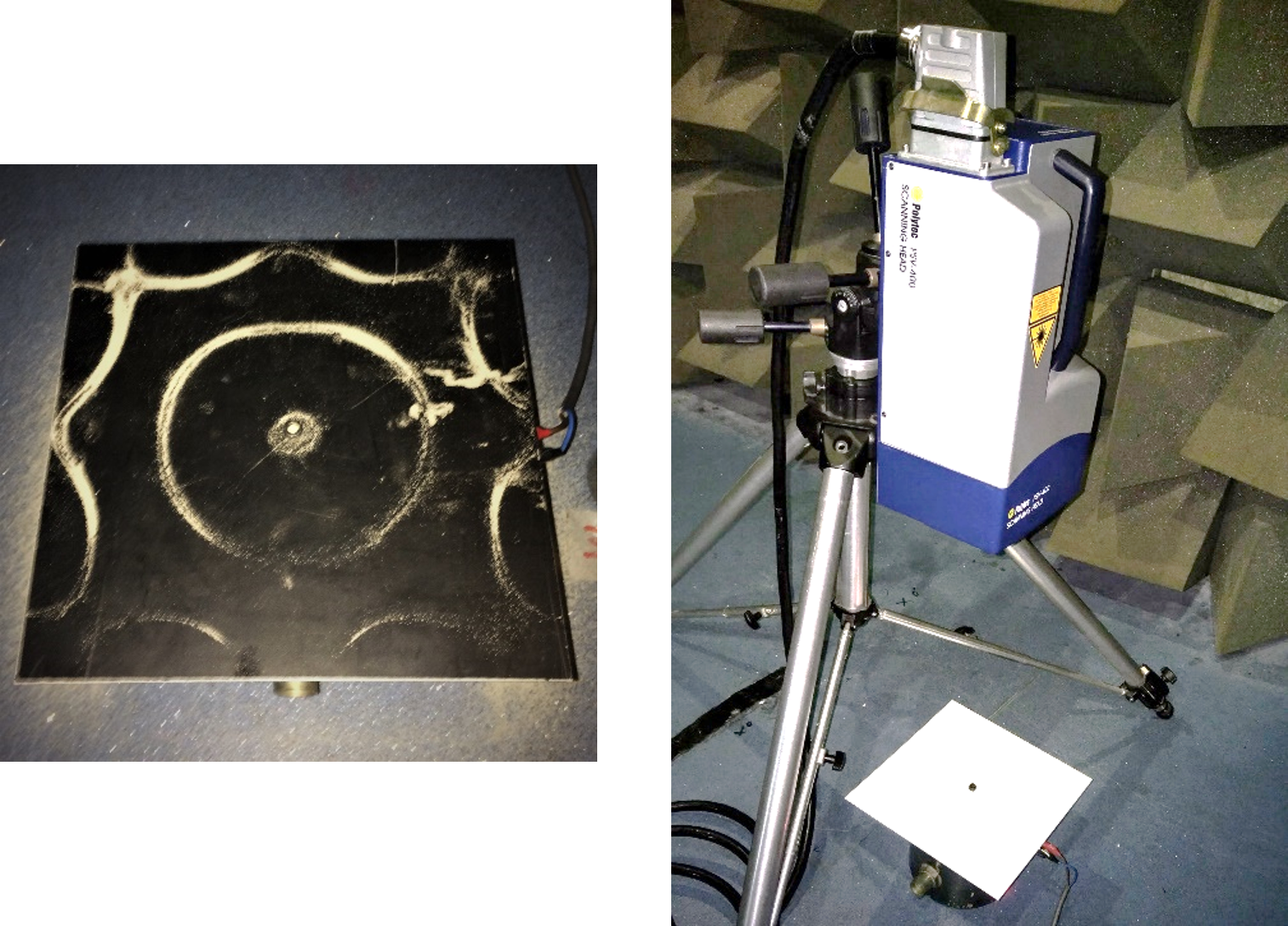
Fig. 3 Chladni plate Measurement. Image credit: Jonathan Hargreaves

Simulated

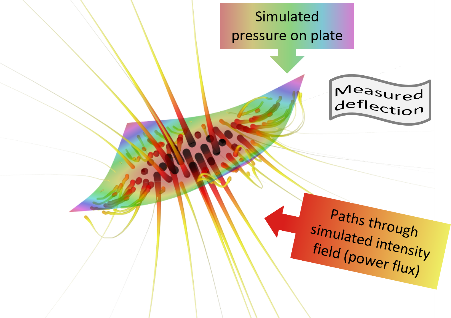
Fig. 4 Chladni plate Simulation. Image credit: Jonathan Hargreaves. Produced using COMSOL Multiphysics™